Beginner Recommender Systems: Episode 5
Now that we have written and run several flows, we can use Metaflow's Client API as a handy way to fetch results, analyze performance and decide how to iterate on embeddings, modeling approaches, and experiment design. You can follow along in this notebook as we load and analyze flow results, and then use TSNE to produce a data visualization.
1Access results with Metaflow's client API
First we import the packages we need and define some config variables:
from metaflow import Flow
import numpy as np
from random import choice
import matplotlib.pyplot as plt
from collections import Counter
from sklearn.manifold import TSNE
FLOW_NAME = 'RecSysTuningFlow'
Let's retrieved the artifacts from the latest successful run.
The get_latest_successful_run uses the metaflow.Flow object to get results of runs using the (class) name of your flows.
def get_latest_successful_run(flow_name: str):
    "Gets the latest successful run."
    for r in Flow(flow_name).runs():
        if r.successful:
            return r
latest_run = get_latest_successful_run(FLOW_NAME)
latest_model = latest_run.data.final_vectors
latest_dataset = latest_run.data.final_dataset
First, check all is in order by printing out datasets and rows and stats:
latest_dataset.head(3)
| playlist_id | artist_sequence | track_sequence | track_test_x | track_test_y | predictions | hit | |
|---|---|---|---|---|---|---|---|
| 56437 | 69080ca9b4d90cc7c6425ccc32626df7-Arcade Fire -... | [Arcade Fire, Arcade Fire, Arcade Fire, Arcade... | [Arcade Fire|||Afterlife, Arcade Fire|||Awful ... | [Arcade Fire|||Afterlife, Arcade Fire|||Awful ... | Arcade Fire|||You Already Know | [Nick Cave & The Bad Seeds|||We No Who U R, Pa... | 0 |
| 9442 | 0a94b98aa949dbb6c9acfd78a79671e2-Double Jointed | [Mark Kozelek, Sun Kil Moon, The Flaming Lips,... | [Mark Kozelek|||Around and Around, Sun Kil Moo... | [Mark Kozelek|||Around and Around, Sun Kil Moo... | Mojave 3|||Writing to St. Peter | [Alexandre Desplat|||Mr. Fox In The Fields Med... | 0 |
| 96621 | 1954a8f3f1a377582fd9b21db7301d32-Joel | [Death Cab for Cutie, Ben Folds Five, Real Est... | [Death Cab for Cutie|||A Lack Of Color, Ben Fo... | [Death Cab for Cutie|||A Lack Of Color, Ben Fo... | Ben Folds|||Zak and Sara | [tUnE-yArDs|||You Yes You, Perfume Genius|||Yo... | 0 |
len(latest_dataset)
2Iterate and improve models in a notebook
Now, let's turn our attention to the model - the embedding space we trained: let's check how big it is and use it to make a test prediction.
print("# track vectors in the space: {}".format(len(latest_model)))
test_track = choice(list(latest_model.index_to_key))
print("Example track: '{}'".format(test_track))
test_vector = latest_model[test_track]
print("Test vector for '{}': {}".format(test_track, test_vector[:5]))
test_sims = latest_model.most_similar(test_track, topn=3)
print("Similar songs to '{}': {}".format(test_track, test_sims))
The skip-gram model we trained is an embedding space: if we did our job correctly, the space is such that tracks closer in the space are actually similar, and tracks that are far apart are pretty unrelated.
Judging the quality of "fantastic embeddings" is hard, but we point here to some common qualitative checks you can run.
# qualitative check, make sure to change with a song that is in the set
test_track = 'Daft Punk|||Get Lucky - Radio Edit'
test_sims = latest_model.most_similar(test_track, topn=3)
print("Similar songs to '{}': {}".format(test_track, test_sims))
If you use 'Daft Punk|||Get Lucky - Radio Edit' as the query item in the space, you will discover a pretty interesting phenomenon, that is, that there are unfortunately many duplicates in the datasets, that is, songs which are technically different but semantically the same, i.e. Daft Punk|||Get Lucky - Radio Edit vs Daft Punk|||Get Lucky.
This is a problem as i) working with dirty data may be misleading, and ii) these issues make data sparsity worse, so the task for our model is now harder. That said, it is cool that KNN can be used to quickly identify and potentially remove duplicates, depending on your dataset and use cases.
Let's map some tracks to known categories: the intuition is that songs that are similar will be colored in the same way in the chart, and so we will expect them to be close in the embedding space.
track_sequence = latest_dataset['track_sequence']
songs = [item for sublist in track_sequence for item in sublist]
song_counter = Counter(songs)
# we downsample the vector space a bit to the K most common songs to avoid crowding the plot / analysis
TOP_N_TRACKS = 250
top_tracks = [_[0] for _ in song_counter.most_common(TOP_N_TRACKS)]
tracks = [_ for _ in latest_model.index_to_key if _ in top_tracks]

assert TOP_N_TRACKS == len(tracks)
# 0 is the generic "unnamed" category
tracks_to_category = {t: 'unknown' for t in tracks}
# we tag songs based on keywords found in the playlist name. Of course, better heuristics are possible ;-)
all_playlists_names = set(latest_dataset['playlist_id'].apply(lambda r: r.split('-')[1].lower().strip()))
target_categories = [
    'rock',
    'rap',
    'country',
    'dance',
    'house'
]
# while not pretty, this select the playlists with the target keyword, and mark the tracks
# as belonging to that category

def tag_tracks_with_category(_df, target_word, tracks_to_category):
    _df = _df[_df['playlist_id'].str.contains(target_word)]
    # debug
    print(len(_df))
    # unnest the list
    songs = [item for sublist in _df['track_sequence'] for item in sublist]
    for song in songs:
        if song in tracks_to_category and tracks_to_category[song] == 'unknown':
            tracks_to_category[song] = target_word

    return tracks_to_category


for cat in target_categories:
    print("Processing {}".format(cat))
    tracks_to_category = tag_tracks_with_category(latest_dataset, cat, tracks_to_category)
Note: to visualize a n-dimensional space, we need to be in 2D. We can use a dimensionality reduction technique like TSNE for this.
def tsne_analysis(embeddings, perplexity=50, n_iter=1000):
    """
    TSNE dimensionality reduction of track embeddings - it may take a while!
    """
    tsne = TSNE(n_components=2, perplexity=perplexity, n_iter=n_iter, verbose=1, learning_rate='auto', init='random')

    return tsne.fit_transform(embeddings)
# add all the tagged tracks to the embedding space, on top of the popular tracks
for track, cat in tracks_to_category.items():
    # add a track if we have a tag, if not there already, if we have a vector for it
    if cat in target_categories and track in latest_model.index_to_key and track not in tracks:
        tracks.append(track)

print(len(tracks))
# extract the vectors from the model and project them in 2D
embeddings = np.array([latest_model[t] for t in tracks])
# debug, print out embedding shape
print(embeddings.shape)
tsne_results = tsne_analysis(embeddings)
assert len(tsne_results) == len(tracks)
Now we can define a function to plot the 2D representations produced by the TSNE algorithm.
def plot_scatterplot_with_lookup(
    title: str,
    items: list,
    items_to_target_cat: dict,
    vectors: list,
    output_path: str = './song_TSNE.png',
    colors = ['#FFE5C7', '#FAAB4A', '#222A30', '#2A679D', '#DCF1FC']
):
    """
    Plot the 2-D vectors in the space, and use the mapping items_to_target_cat
    to color-code the points for convenience
    """

    colors = iter(colors)

    plt.ioff()

    groups = {}
    for item, target_cat in items_to_target_cat.items():
        if item not in items:
            continue

        item_idx = items.index(item)
        x = vectors[item_idx][0]
        y = vectors[item_idx][1]
        if target_cat in groups:
            groups[target_cat]['x'].append(x)
            groups[target_cat]['y'].append(y)
        else:
            groups[target_cat] = {
                'x': [x], 'y': [y]
            }

    fig, ax = plt.subplots(figsize=(6,6))
    for i, (group, data) in enumerate(groups.items()):
        color = 'k' if group == 'unknown' else next(colors)
        ax.scatter(data['x'], data['y'],
                   alpha=0.1 if group == 'unknown' else 0.8,
                   edgecolors='none',
                   s=25,
                   marker='o',
                   label=group,
                   color=color)

    [ax.spines[dir].set_visible(False) for dir in ['top', 'bottom', 'left', 'right']]
    ax.set_xticks([])
    ax.set_yticks([])
    plt.title(title)
    plt.legend(loc=2)
    fig.savefig(output_path)
    plt.close()
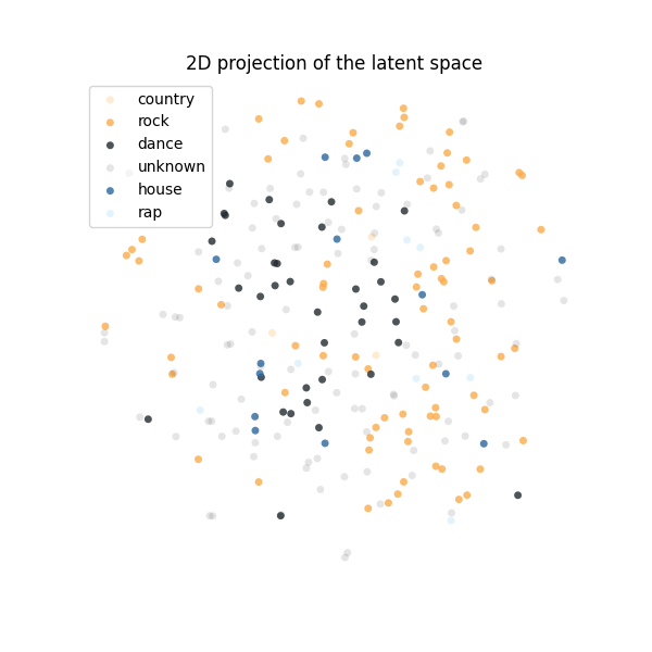
Finally, we are ready to plot the latent space!
plot_scatterplot_with_lookup(
    '2D projection of the latent space',
    tracks,
    tracks_to_category,
    tsne_results)
So far, you have trained embeddings and models, tuned them to find the most promising candidates, and analyzed the results using Metaflow's Client API. In the final episode of this tutorial, we will make another FlowSpec object that shows how you can combine these processes with Sagemaker's convenient deployment tools. The end result will be a recommender system you can use to serve real-time predictions about what song to suggest next to a user of an app. See you there!