Beginner Recommender Systems: Episode 1
Before diving deep into Metaflow, this lesson will introduce our problem and do a preliminary analysis of our dataset. You can follow along in this notebook if you want to run the code yourself. You will learn a little bit about recommender systems, the kinds of data the flow through them, and then you will be introduced to a Spotify playlist dataset that the rest of the tutorial will build a next song recommender system.
1RecSys 101
Recommender systems (RSs) are some of the most ubiquitous ML systems in production: whether Netflix suggesting you what movie to watch, Amazon what books to buy, or Linkedin which data influencer to follow, RSs play a pivotal role in our digital life (it is estimated the RSs market will be around 15BN in 2026!).
The model architecture, and therefore many MLOps choices, of a given RS, depends heavily on the use case. While a full taxonomy is beyond the scope of this tutorial, we can provide a simple taxonomy of RSs based on the type of input and output they process.
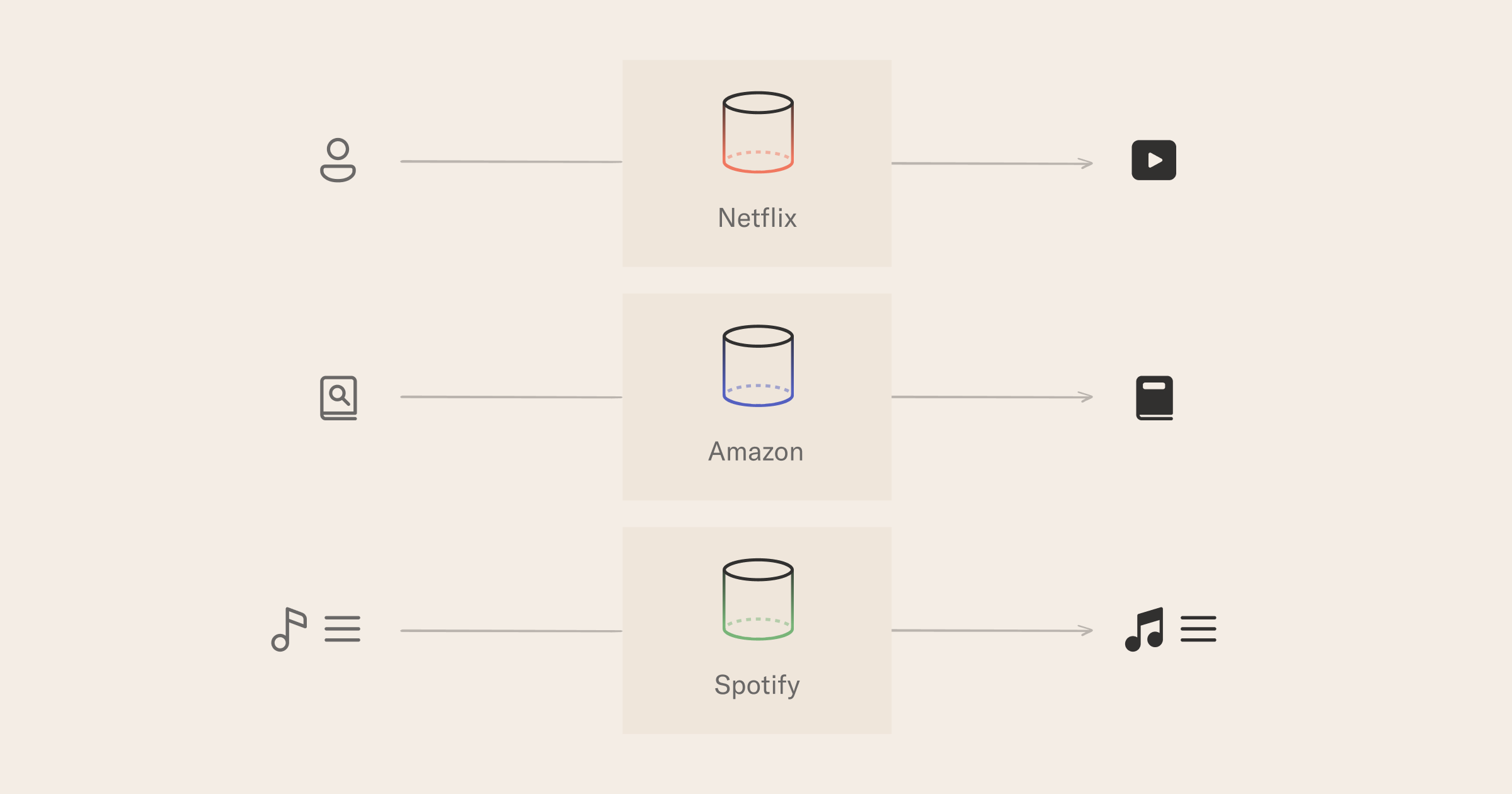
- input user, output item - example: Netflix recommends you a movie that they think you would enjoy;
- input item, output item - example: while browsing a book page, Amazon recommends you another book because "people often look at X as well";
- input a list of items, output the next items - Spotify is picking songs to suggest in your discover weekly playlist based on what songs you have listened to lately.
Finally, as far as input data goes, there is important distinction practitioners make between content and behavioral data.
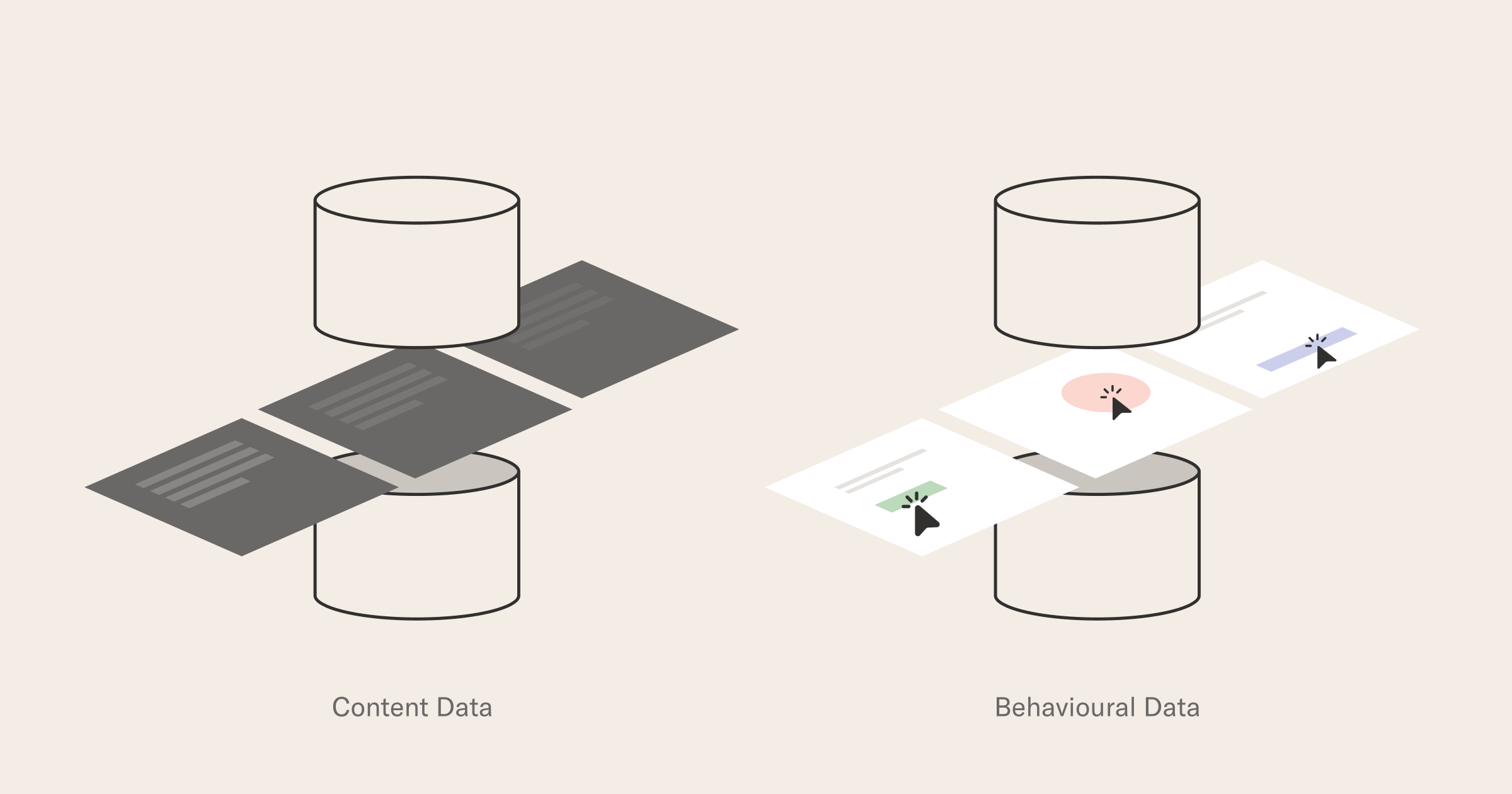
Content data is data that does not depend on any interaction: think for example of the author of a book on Amazon, or a movie poster on Netflix - even if nobody will ever watch that movie, we could still use some basic metadata to decide how likely we are to like it. Behavioral data is the result of user interactions with a system: it may be add-to-cart events for e-commerce or previous people you added on Facebook - generally speaking, behavioral data needs systems in place to capture and store these signals, often under time constraints.
While the general rule of ML applies and more data is better, in practice the use case and modeling technique(s) will constrain what is feasible: for example, if you are building a RS for a completely new product, with 0 or few active users, content-based data is your only option! The trick to building a recommender system for a product is to be able to ship something that is good enough to generate interest in the product, so over time you can build an increasingly useful behavioral dataset as the product improves.
2Next event prediction for songs
Armed with our taxonomy, we can explore what is the use case we are trying to solve today:
Can we suggest what to listen to next when presented with a song?
You will build a sequential recommender system that matches case 3 above. The model will learn from existing sequences (playlists by real users) how to continue extending an arbitrary new list. More generally, this task is also known as next event prediction (NEP). The modeling technique we picked will only leverage behavioral data in the form of interactions created by users when composing their playlists.
The training set is a list of playlists, e.g.:
- song_1, song_414, song_42425
- song_412, song_2214, song_525, song_11, song_414, song_42425
- song_12, song_416
- ...
The key intuition about our modeling is that "songs that often appear in similar contexts" are similar. If we observe that "Imagine" and "Hey Jude" tend to appear in similar playlists, they must have something in common!
At prediction time, our input will be an unseen playlist with N songs: we will take the first N - 1 songs as the input (or query) for our model, and ask it to predict the last, missing item, that is:
- song_525, song_22, song_814, song_4255
will become:
- query: song_525, song_22, song_814
- label: song_4255
If our model is able to guess "song_4255", we will count it as a successful prediction. Of course, we have left all the juicy details out - so no worries if things feel a bit vague: for now, we just want to be very clear about what problem we are solving, and which type of input/output data our model should deal with.
In the rest of the notebook, we will read our dataset and start getting familiar with the main entities of characters of our story, tracks, and playlists.
3Download the dataset
You can download the dataset from Kaggle here.
Place the downloaded file in the recsys directory and unzip it.
unzip ./archive.zip
rm ./archive.zip
We need to do so minor data cleaning, which can be handled by running the following script.
python clean_dataset.py
4What does the data look like?
Before loading the data, there are a few packages to import:
import pandas as pd
import matplotlib.pyplot as plt
from collections import Counter
import powerlaw
Now we can load the dataset and explore its structure. The dataset is stored in a .parquet file. Loading parquet files into dataframes is a common pattern when working with large tabular datasets like the kind often found in RSs. If you are curious, we have a post all about common file formats for tabular datasets.
df = pd.read_parquet('cleaned_spotify_dataset.parquet')
df.head(3)
| row_id | user_id | artist | track | playlist | |
|---|---|---|---|---|---|
| 0 | 0 | 9cc0cfd4d7d7885102480dd99e7a90d6 | Elvis Costello | (The Angels Wanna Wear My) Red Shoes | HARD ROCK 2010 |
| 1 | 1 | 9cc0cfd4d7d7885102480dd99e7a90d6 | Elvis Costello & The Attractions | (What's So Funny 'Bout) Peace, Love And Unders... | HARD ROCK 2010 |
| 2 | 2 | 9cc0cfd4d7d7885102480dd99e7a90d6 | Tiffany Page | 7 Years Too Late | HARD ROCK 2010 |
How many data samples are there?
len(df)
What artists and songs are most popular?
artist_counter = Counter(list(df['artist']))
song_counter = Counter(list(df['track']))
print("\nTop artists: {}\n".format(artist_counter.most_common(20)))
print("\nTop songs: {}\n".format(song_counter.most_common(20)))
Let's visualize the distribution of tracks and artist in our dataset.
def plot_distribution(artists, tracks, n_bins: int=50, outpath = './artist-track-dist.png'):
    """
    Plot distributions of tracks and artists in the final dataset.
    """
    import numpy as np
    from itertools import product
    import seaborn as sns
    sns.set_style()
    import matplotlib.pyplot as plt
    plt.ioff()
    fig, axs = plt.subplots(1, 2, tight_layout=True, figsize=(8,4))
    axs[0].hist(artist_counter.values(), bins=n_bins, color='#2E3454')
    axs[0].set_title('Artists', fontsize=16)
    axs[0].set_yscale('log')
    axs[0].ticklabel_format(axis="x", style="sci", scilimits=(0,0))
    axs[0].set_xlabel('# of artists')
    axs[0].set_ylabel('# of times artist is in a playlist')
    axs[1].hist(song_counter.values(), bins=n_bins, color='#2E3454')
    axs[1].set_title('Songs', fontsize=16)
    axs[1].set_yscale('log')
    axs[1].ticklabel_format(axis="x", style="sci", scilimits=(0,0))
    axs[1].set_xlabel('# of songs')
    axs[1].set_ylabel('# of times song is in a playlist')
    for (i,side) in list(product([0,1], ['top', 'right'])):
        axs[i].spines[side].set_visible(False)
    fig.savefig(outpath)
    plt.close()
    return
plot_distribution(artist_counter, song_counter);
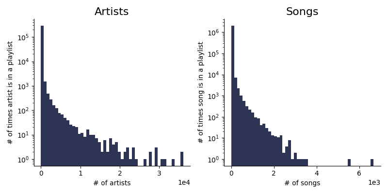
Since it looks like our data is very skewed, we can use the powerlaw library and formally compare the distribution of how artists are represented in playlists to a powerlaw. Specifically, we use the package to visualize the probability density function for the theoretical distribution estimated using the number of times artists are represented in playlists.
data = list(artist_counter.values())
fit = powerlaw.Fit(data, discrete=True)
fig, ax = plt.subplots(1,1,figsize=(4,4))
ax.spines['top'].set_visible(False)
ax.spines['right'].set_visible(False)
data = list(artist_counter.values())
fit = powerlaw.Fit(data, discrete=True)
figCCDF = fit.plot_pdf(color='#2E3454', linewidth=2, ax=ax)
fit.power_law.plot_pdf(color='#2E3454', linestyle='--', ax=figCCDF)
fig.savefig('./powerlaw.png');
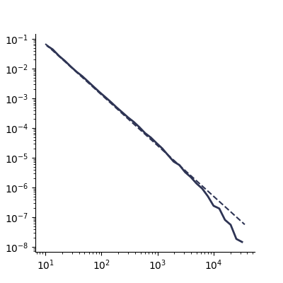
Nice work! In this lesson, you explored a dataset with millions of Spotify songs and their playlist groupings. You saw which artists and songs are most popular and observed how the distribution of how artists are represented in playlists follows a power law. In the next episode, we will see how to leverage DuckDB to query the dataset efficiently. See you there!