Intermediate Recommender Systems: Episode 1
1What is the machine learning? 🤖🧠
In particular, in this tutorial we use the H&M dataset to reproduce a classic user-item, offline training-offline serving recommendation use case, that is:
- user-item: at test time, our model will receive a user identifier as the query, and will be tasked with suggesting k (fashion) items that she is likely to buy. Since we have ground truth for past behavior, we can use previous purchases to test our model generalization abilities as we train it;
- offline training-offline serving: we assume our shoppers are, for the vast part, constants - that will allow us to build a pipeline that runs Monday night, makes k predictions for each user based on the data we have so far and stores those predictions in a cache. While not all use cases can be solved in this way, offline serving is a powerful pattern: a major benefit of this approach is that recommendations can be served with very low latency at a massive scale while maintaining high availability. This pattern is used by some of the most popular recommenders in the industry, such as movie recommendations at Netflix.com. For an example of offline training and online serving, you could check the end of our previous tutorial.
2Download the data ⬇️
The original dataset is here. Download and unzip these three .csv files:
articles.csvcustomers.csvtransactions_train.csv
Then run create_parquet_dataset.py to obtain the basic parquet files for the flow. If you have concerns about your laptop capabilities, or you later run in to an Out of Memory Error, you can change the single argument of this script, which is a number between 0 and 1 that specifies the fraction of the original data you want to use in the downstream workflow.
python create_parquet_dataset.py 0.25
The result will of running this script will produce three parquet files, corresponding to each of the .csv files you downloaded.
articlescustomerstransactions_train
3Setup dbt profile and transform raw data
Now we want to run transformations on the parquet files.
To simplify the downstream machine learning flow, we run data transformation before starting the flow in this example. If you want, you can also incorporate the transformation code in a flow, as demonstrated in this project, and explained in previous Outerbounds posts.
Motivation: Why use DuckDB in the transformation layer?
In this tutorial, will use the dbt DuckDB extension to run our directed acyclic graph (DAG) of transformations using DuckDB as a fast local analytic engine. This runs our transformations locally, in lieu of running transformations in a data warehouse. Using DuckDB in this way affords extremely powerful workflows for enterprise data scientists, where changing from a flexible local setup to a robust production environment becomes a simple config change.
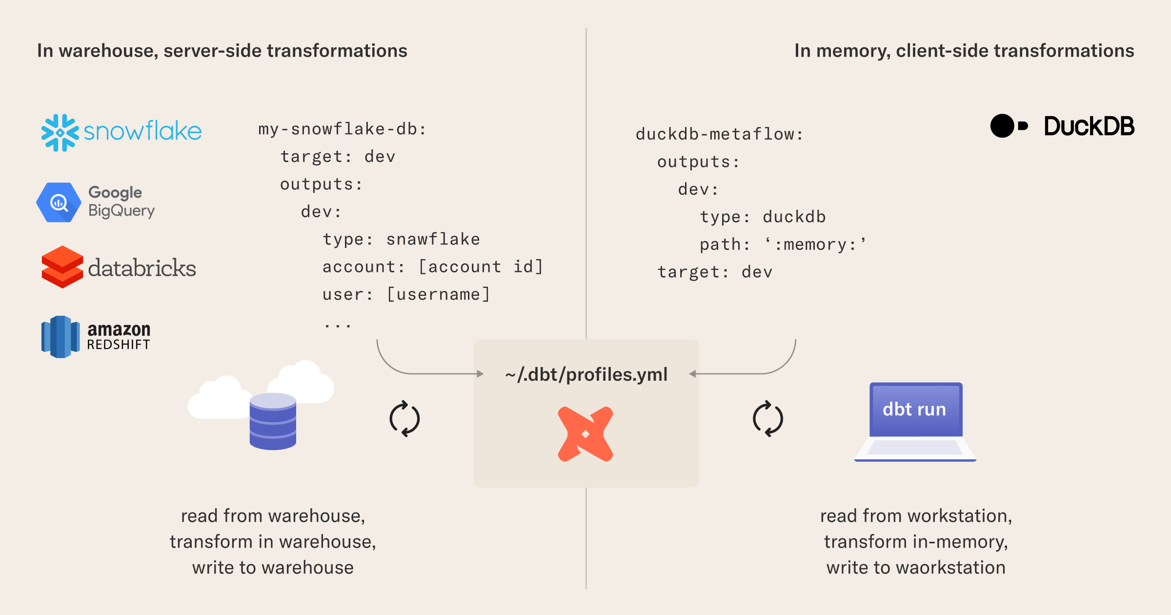
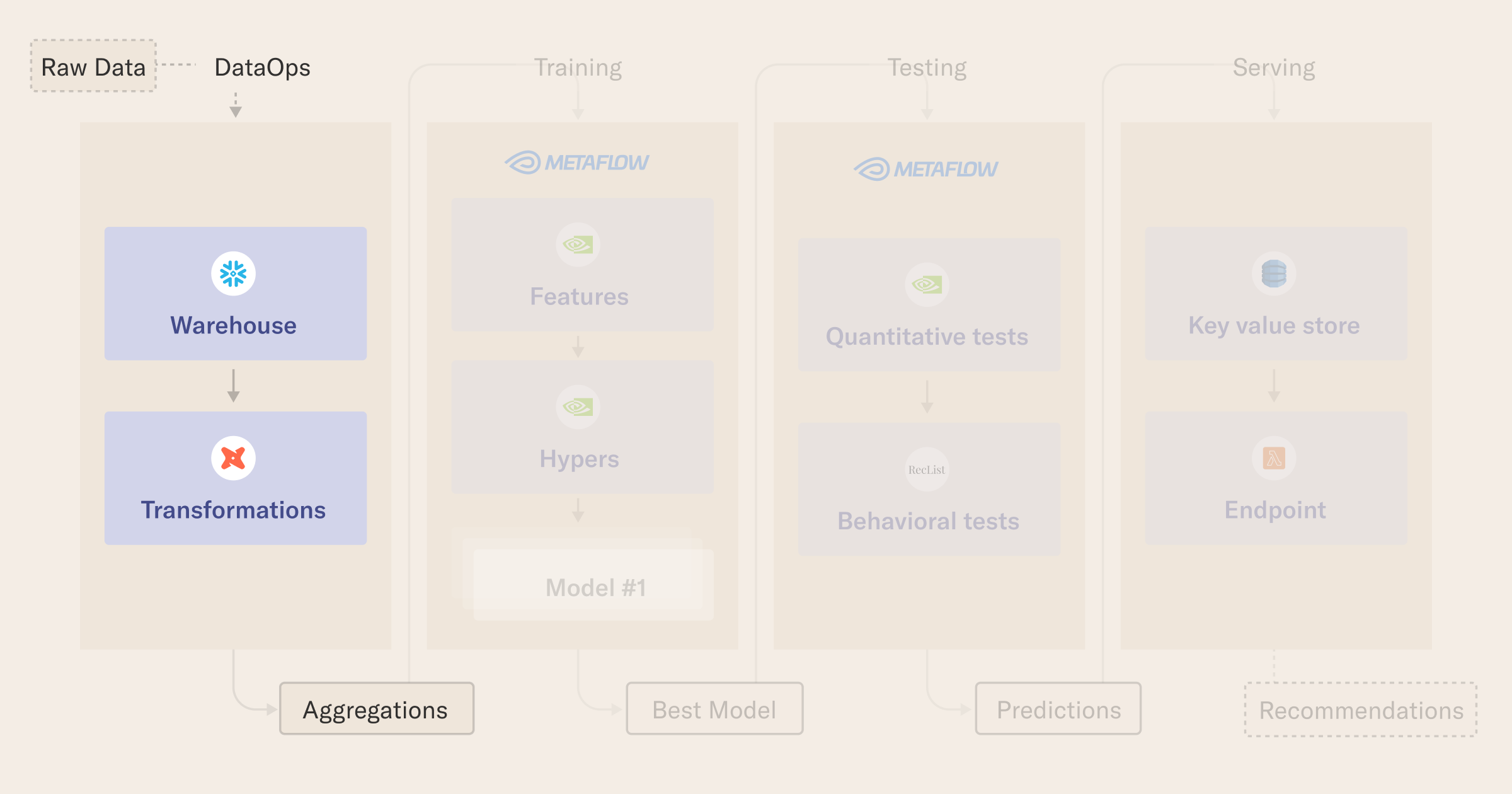
Running dbt transformations locally with DuckDB means we only need to change dbt profiles to run the transformations on a full-sized production dataset in a data warehouse like Snowflake or BigQuery. Later, you will see how Metaflow extends this parity between training and production environments to a full machine learning stack, making the dbt, DuckDB, and Metaflow combination a lean and portable toolchain for developing data-intensive applications.
Setup
To setup your duckdb-metaflow profile for dbt (you can pick another profile name if you want, the key here is the type and path sections), add the following in ~/.dbt/profiles.yml:
duckdb-metaflow:
  outputs:
   dev:
     type: duckdb
     path: ':memory:'
  target: dev
In our example, the dbt_project.yml file in your working directory is already configured to use the profile when running the project.
To use it:
- cd into the
dbtfolder; dbt runwill run the SQL transformations and produce the final output we need for our Python flow!
cd dbt
dbt run
You can check that dbt ran the DAG successfully by seeing if a filtered_dataframe.parquet gets created in the project folder at the end - this contains the table we need, with all the data pre-joined, to run the flow.
If you see an Out of Memory Error, return to section 1 of this page and select a lower number as the argument to the create_parquet_dataset.py script. This number in between 0 to 1 is proportional to the size of the filtered_dataframe.parquet output.
4Query the data with DuckDB
In the DataPrepFlow, you will see how to query the filtered_dataframe.parquet file using DuckDB, so it is usable in downstream steps.
The objective is to run a SQL query that produces three PyArrow tables for training, validation, and test dataset.
Our final table is a wide, flat dataset containing a transaction for each row. A transaction is minimally defined by a timestamp, the ID of the customer, and the ID of the product. However, to leverage the power of the two-tower model you will meet in the next lesson of this tutorial we also report meta-data for the customer and the product, hoping this will facilitate the learning of better embeddings.
from metaflow import FlowSpec, step, batch, Parameter, current
from datetime import datetime

class DataPrepFlow(FlowSpec):

    ### DATA PARAMETERS ###
    ROW_SAMPLING = Parameter(
        name='row_sampling',
        help='Row sampling: if 0, NO sampling is applied. Needs to be an int between 1 and 100',
        default='1'
    )

    # NOTE: data parameters - we split by time, leaving the last two weeks for validation and tests
    # The first date in the table is 2018-09-20
    # The last date in the table is 2020-09-22
    TRAINING_END_DATE = Parameter(
        name='training_end_date',
        help='Data up until this date is used for training, format yyyy-mm-dd',
        default='2020-09-08'
    )

    VALIDATION_END_DATE = Parameter(
        name='validation_end_date',
        help='Data up after training end and until this date is used for validation, format yyyy-mm-dd',
        default='2020-09-15'
    )

    @step
    def start(self):
        """
        Start-up: check everything works or fail fast!
        """
        # print out some debug info
        print("flow name: %s" % current.flow_name)
        print("run id: %s" % current.run_id)
        print("username: %s" % current.username)
        # we need to check if Metaflow is running with remote (s3) data store or not
        from metaflow.metaflow_config import DATASTORE_SYSROOT_S3
        print("DATASTORE_SYSROOT_S3: %s" % DATASTORE_SYSROOT_S3)
        if DATASTORE_SYSROOT_S3 is None:
            print("ATTENTION: LOCAL DATASTORE ENABLED")
        # check variables and connections are working fine
        assert int(self.ROW_SAMPLING)
        # check the data range makes sense
        self.training_end_date = datetime.strptime(self.TRAINING_END_DATE, '%Y-%m-%d')
        self.validation_end_date = datetime.strptime(self.VALIDATION_END_DATE, '%Y-%m-%d')
        assert self.validation_end_date > self.training_end_date

        self.next(self.get_dataset)

    @step
    def get_dataset(self):
        """
        Get the data in the right shape using duckDb, after the dbt transformation
        """
        from pyarrow import Table as pt
        import duckdb
        # check if we need to sample - this is useful to iterate on the code with a real setup
        # without reading in too much data...
        _sampling = int(self.ROW_SAMPLING)
        sampling_expression = '' if _sampling == 0 else 'USING SAMPLE {} PERCENT (bernoulli)'.format(_sampling)
        # thanks to our dbt preparation, the ML models can read in directly the data without additional logic
        query = """
            SELECT
                ARTICLE_ID,
                PRODUCT_CODE,
                PRODUCT_TYPE_NO,
                PRODUCT_GROUP_NAME,
                GRAPHICAL_APPEARANCE_NO,
                COLOUR_GROUP_CODE,
                PERCEIVED_COLOUR_VALUE_ID,
                PERCEIVED_COLOUR_MASTER_ID,
                DEPARTMENT_NO,
                INDEX_CODE,
                INDEX_GROUP_NO,
                SECTION_NO,
                GARMENT_GROUP_NO,
                ACTIVE,
                FN,
                AGE,
                CLUB_MEMBER_STATUS,
                CUSTOMER_ID,
                FASHION_NEWS_FREQUENCY,
                POSTAL_CODE,
                PRICE,
                SALES_CHANNEL_ID,
                T_DAT
            FROM
                read_parquet('filtered_dataframe.parquet')
                {}
            ORDER BY
                T_DAT ASC
        """.format(sampling_expression)
        print("Fetching rows with query: \n {} \n\nIt may take a while...\n".format(query))
        # fetch raw dataset
        con = duckdb.connect(database=':memory:')
        con.execute(query)
        dataset = con.fetchall()
        # convert the COLS to lower case (Keras does complain downstream otherwise)
        cols = [c[0].lower() for c in con.description]
        dataset = [{ k: v for k, v in zip(cols, row) } for row in dataset]
        # debug
        print("Example row", dataset[0])
        self.item_id_2_meta = { str(r['article_id']): r for r in dataset }
        # we split by time window, using the dates specified as parameters
        # NOTE: we could actually return Arrow table directly, by then running three queries over
        # a different date range (e.g. https://duckdb.org/2021/12/03/duck-arrow.html)
        # For simplicity, we kept here the original flow compatible with warehouse processing
        train_dataset = pt.from_pylist([row for row in dataset if row['t_dat'] < self.training_end_date])
        validation_dataset = pt.from_pylist([row for row in dataset
            if row['t_dat'] >= self.training_end_date and row['t_dat'] < self.validation_end_date])
        test_dataset = pt.from_pylist([row for row in dataset if row['t_dat'] >= self.validation_end_date])
        print("# {:,} events in the training set, {:,} for validation, {:,} for test".format(
            len(train_dataset),
            len(validation_dataset),
            len(test_dataset)
        ))
        # store and version datasets as a map label -> datasets, for consist processing later on
        self.label_to_dataset = {
            'train': train_dataset,
            'valid': validation_dataset,
            'test': test_dataset
        }
        # go to the next step for NV tabular data
        self.next(self.end)

    @step
    def end(self):
        """
        Just say bye!
        """
        print("All done\n\nSee you, recSys cowboy\n")
        return

if __name__ == '__main__':
    DataPrepFlow()
5Run your flow ▶️
python data_prep.py run
If this flow ran successfully, you have already done a lot! You now have a workflow that you can use to keep data transformation workflows in perfect parity locally and in your production warehouse(s). Moreover, you have built a solid foundation to start leveraging the power of Metaflow to extend this workflow by building and deploying complex models. Click through to the next lesson to start building up your recommender system training loop.