Intermediate Computer Vision: Episode 1
Introduction
In this tutorial, you will build an image classifier on a large image dataset. You will learn how to move large amounts of data between your local environment, S3 storage, and remote compute instances where models are trained. You will fine-tune state-of-the-art model architectures on cloud GPUs and track results with Tensorboard. Before diving into these details, let's meet the dataset we will use to guide the tutorial.
This tutorial has six episodes. If you want to run the code, you can follow along with this first page in this Jupyter notebook.
1What is the HaGRID Dataset?
HaGRID is a large image dataset with labels and annotations for classification or detection tasks. The full HaGRID dataset is 716GB with 552,992 images divided into 18 classes of hand gestures. Conveniently, the authors provide an evenly split (by class) 2GB sample that leads to cloud runs you can complete in one sitting. You can find more details in the GitHub repository and corresponding paper, HaGRID - HAnd Gesture Recognition Image Dataset.
2Download the Data
You can use wget to download the subsample data from the URLs provided by the authors. The subsample will download 100 images from each class. Run the following from the command line to fetch the zipped data and place the zip file in the data directory.
mkdir data && wget 'https://sc.link/AO5l' -O 'data/subsample.zip'
Then you can unzip the resulting subsample.zip file.
unzip -qq 'data/subsample.zip' -d 'data/subsample'
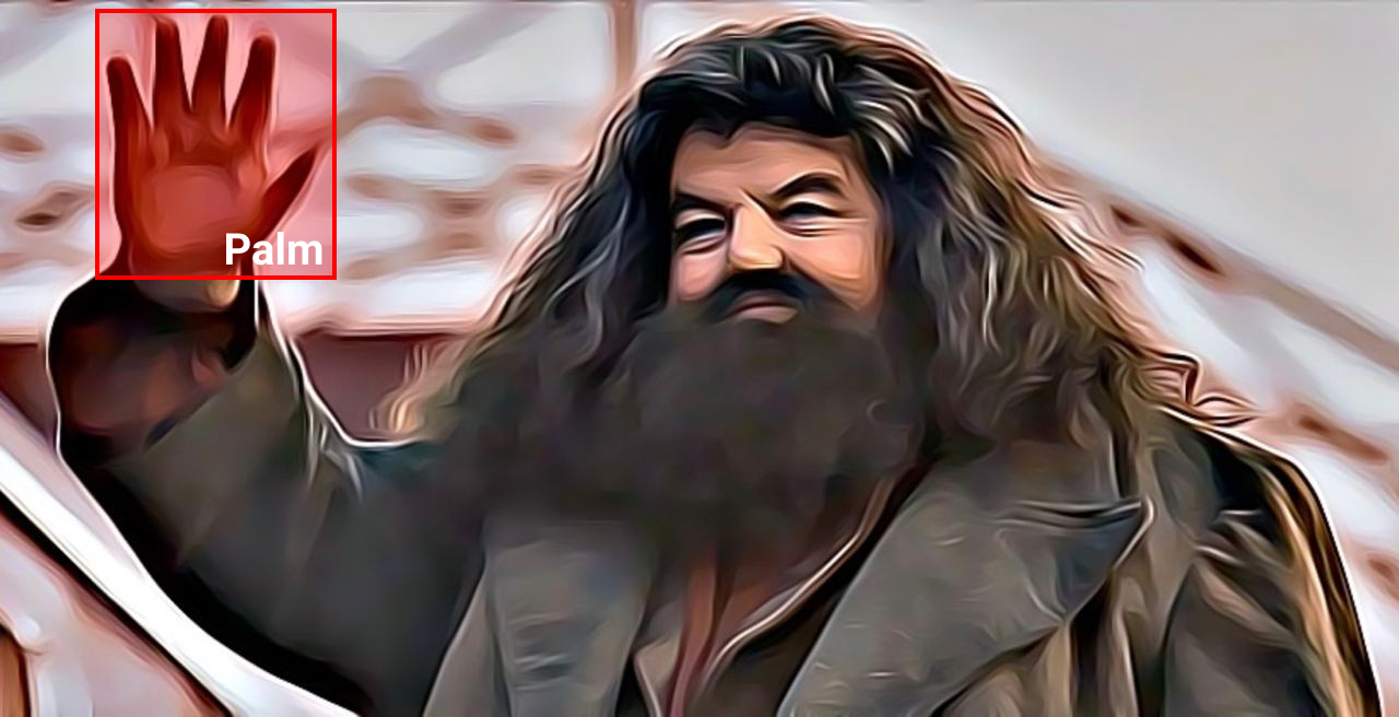
3View Sample Images
Let's look at one class of images. You can see the available gesture labels by looking at the directories created when you unzipped the subsample.
ls 'data/subsample'
In the next cell, pick a gesture variable from one of the 18 dataset labels.
relative_data_path = 'data/subsample'
gesture = 'peace'
Then we can grab sample images from the corresponding folder and visualize the result:
import os
import glob
import random
import matplotlib.pyplot as plt
from PIL import Image


N_IMAGES = 3
AX_DIM = 3
path = (os.getcwd(), relative_data_path, gesture, '*.jpg')
sample_images = random.sample(glob.glob(os.path.join(*path)), N_IMAGES)
plt.ioff()
fig, axes = plt.subplots(
    1, len(sample_images),
    figsize = (AX_DIM * len(sample_images), AX_DIM)
)
fig.tight_layout()

for img, ax in zip(sample_images, axes):

    # configure axis
    ax.spines['right'].set_visible(False)
    ax.spines['left'].set_visible(False)
    ax.spines['top'].set_visible(False)
    ax.spines['bottom'].set_visible(False)
    ax.set_xticks([])
    ax.set_yticks([])

    # display image
    ax.imshow(Image.open(img))

fig.savefig(fname='{}-sample.png'.format(gesture));

Similar to the command to download the images, you can download annotations using wget:
wget 'https://sc.link/EQ5g' -O 'data/subsample-annotations.zip'
 unzip -qq 'data/subsample-annotations.zip'  -d 'data/subsample-annotations'
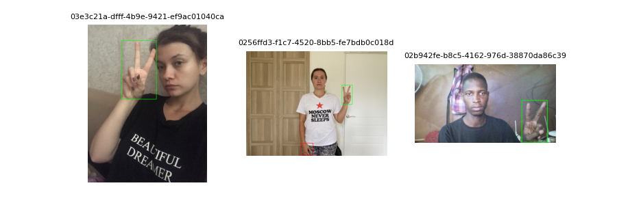
Let's inspect the annotations.
The following code will draw a green box around the gesture of interest and a red box around other hands labeled in the image that are not making a gesture.
These boxes correspond to the bboxes property that comes with each image annotation.
import json
import cv2

relative_annotation_path = 'data/subsample-annotations/ann_subsample/{}.json'.format(gesture)
result = json.load(open(relative_annotation_path))

color = None
AX_DIM = 3
plt.ioff()
fig, axes = plt.subplots(1, len(sample_images), figsize = (AX_DIM * len(sample_images), AX_DIM))

for im_file, ax in zip(sample_images, axes):

    # get image
    img_key = im_file.split('/')[-1].split('.')[0]
    image = cv2.imread(im_file)

    # openCV dims are BGR
    b,g,r = cv2.split(image)
    image = cv2.merge([r,g,b])

    # fetch bounding box for gesture
    for i, label in enumerate(result[img_key]['labels']):

        # determine annotation type
        if label == gesture:
            color = (0, 255, 0)
        elif label == 'no_gesture':
            color = (255, 0, 0)

        # unpack annotation format
        bbox = result[img_key]['bboxes'][i]
        top_left_x, top_left_y, w, h = bbox
        scale_x = image.shape[1]
        scale_y = image.shape[0]

        # draw bounding box to image scale
        x1 = int(top_left_x * scale_x)
        y1 = int(top_left_y * scale_y)
        x2 = int(x1 + scale_x * w)
        y2 = int(y1 + scale_y * h)
        cv2.rectangle(image, (x1, y1), (x2, y2), color, thickness=3)

        # display image
        ax.imshow(image)

    # configure axis
    ax.spines['right'].set_visible(False)
    ax.spines['left'].set_visible(False)
    ax.spines['top'].set_visible(False)
    ax.spines['bottom'].set_visible(False)
    ax.set_xticks([])
    ax.set_yticks([])
    ax.set_title(img_key, fontsize=8)

fig.savefig('{}-sample-bbox.png'.format(gesture))
4A Baseline Gesture Classification Model
The learning task of interest in this tutorial is to classify images by gesture.
In the previous section, you saw that each image comes with a gesture label and a bounding box in the corresponding annotation.
Let's build a baseline model to predict the gesture for each image.
We use the majority-class classifier, which measures what happens when we predict all of examples in the test set with the majority class.
First, lets load the dataset using PyTorch objects you will learn about in the next episode.
import torch
from hagrid.classifier.dataset import GestureDataset
from hagrid.classifier.preprocess import get_transform
from hagrid.classifier.utils import collate_fn
from omegaconf import OmegaConf
from torch import nn, Tensor

path_to_config = './hagrid/classifier/config/default.yaml'
conf = OmegaConf.load(path_to_config)
N_CLASSES = 19

test_dataset = GestureDataset(is_train=False, conf=conf, transform=get_transform())
test_dataloader = torch.utils.data.DataLoader(
    test_dataset,
    batch_size=conf.train_params.test_batch_size,
    num_workers=conf.train_params.num_workers,
    shuffle='random',
    collate_fn=collate_fn,
    persistent_workers = True,
    prefetch_factor=conf.train_params.prefetch_factor,
)
criterion = nn.CrossEntropyLoss()
Then let's check the performance of the baseline model (always predict class 0) on one pass through the test set.
Next, we collect the true targets next to compare to our benchmark approach.
from collections import defaultdict

targets = defaultdict(list)
n_targets_seen = defaultdict(int)
for i, (images, labels) in enumerate(test_dataloader):
    accuracies = {target:[] for target in list(labels)[0].keys()}
    for target in list(labels)[0].keys():
        target_labels = [label[target] for label in labels]
        targets[target] += target_labels
        n_targets_seen[target] += len(target_labels)

target = 'gesture'
targets = torch.tensor(targets[target], dtype=torch.int32)
predicts_labels = torch.zeros(n_targets_seen[target], dtype=torch.int32)
Finally, we compute metric scores that we will be tracking on data subsets that we evaluate at the end of each epoch.
from torchmetrics.functional import accuracy, f1_score, precision, recall, auroc, confusion_matrix
num_classes = 19
average = conf.metric_params["average"]
metrics = conf.metric_params["metrics"]
scores = {
    "accuracy": accuracy(predicts_labels, targets, average=average, num_classes=num_classes).item(),
    "f1_score": f1_score(predicts_labels, targets, average=average, num_classes=num_classes).item(),
    "precision": precision(predicts_labels, targets, average=average, num_classes=num_classes).item(),
    "recall": recall(predicts_labels, targets, average=average, num_classes=num_classes).item()
}
scores
In our baseline model, we see accuracy somewhere around 5% which makes sense given we have 18 evenly distributed classes.
In this episode, you were introduced to the HaGRID dataset. Each data point is labeled with a class from 18 different hand gesture labels. In the rest of this tutorial, you will learn how to build a computer vision model training workflow to predict hand gesture classes using this data. The next episode starts this journey by introducing the fundamentals of PyTorch data loaders.