Beginner Computer Vision: Episode 3
This episode references this script.
As you scale your machine learning operations, it becomes more important to reuse code across steps and flows. This episode will leverage Metaflow's ability to parallelize the execution of steps in your code. You'll see how to run copies of the same function in cloud compute environments.
1Best Practice: Reusable Code
To integrate the Keras models you have built in a Metaflow flow it is convenient to put them in functions in a Python file such as models.py. In this example we implement the following functions:
make_baseline: Constructs a Keras model like our baseline architecture from episode 1.make_cnn: Construct a Keras model like the CNN architecture from episode 2.fit_and_score: Fit the model and return scores on a validation set.
The functions are grouped together in the ModelOperations class. This class isn't necessary but is shown here to demonstrate a useful pattern to make functions easier to reuse and test. In the next section, you will be introduced to Metaflow by defining the ModelComparisonFlow object, which will use functionality defined by the ModelOperations class.
from tensorflow import keras

class ModelOperations:

    recall = 0.96
    precision = 0.96

    def make_baseline(self):
        model = keras.Sequential()
        model.add(keras.layers.Dense(
            self.num_pixels, input_dim=self.num_pixels,
            kernel_initializer=self.kernel_initializer,
            activation='relu'
        ))
        model.add(keras.layers.Dense(
            self.num_classes,
            kernel_initializer=self.kernel_initializer,
            activation='softmax'
        ))
        model.compile(
            loss=self.loss,
            optimizer=self.optimizer,
            metrics=self._keras_metrics()
        )
        return model

    def make_cnn(
        self,
        hidden_conv_layer_sizes = None
    ):
        model = keras.Sequential()
        if hidden_conv_layer_sizes is None:
            hidden_conv_layer_sizes = self.hidden_conv_layer_sizes
        _layers = [keras.Input(shape=self.input_shape)]
        for conv_layer_size in hidden_conv_layer_sizes:
            _layers.append(keras.layers.Conv2D(
                conv_layer_size,
                kernel_size=self.kernel_size,
                activation="relu"
            ))
            _layers.append(keras.layers.MaxPooling2D(
                pool_size=self.pool_size
            ))
        _layers.extend([
            keras.layers.Flatten(),
            keras.layers.Dropout(self.p_dropout),
            keras.layers.Dense(self.num_classes, activation="softmax")
        ])
        model = keras.Sequential(_layers)
        model.compile(
            loss=self.loss,
            optimizer=self.optimizer,
            metrics=self._keras_metrics()
        )
        return model

    def fit_and_score(self, x_train, x_test):
        history = self.model.fit(
            x_train, self.y_train,
            validation_data = (x_test, self.y_test),
            epochs = self.epochs,
            batch_size = self.batch_size,
            verbose = self.verbose
        )
        scores = self.model.evaluate(x_test, self.y_test, verbose = 0)
        return history, scores

    def _keras_metrics(self):
        keras_metrics = []
        for _m in self.metrics:
            if _m == 'precision at recall':
                keras_metrics.append(
                    keras.metrics.PrecisionAtRecall(recall=self.recall)
                )
            elif _m == 'recall at precision':
                keras.metrics.append(
                    keras.metrics.RecallAtPrecision(precision=self.precision)
                )
            else:
                keras_metrics.append(_m)
        return keras_metrics
2Write a Flow
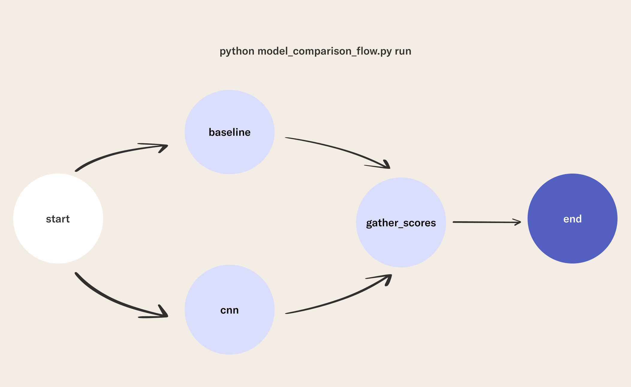
This flow is designed to compare the baseline model against the CNN model. It includes:
- All of the functions defined in the
ModelOperationsclass. - A
startstep where we read the data. - A
baselinestep where the baseline model is fit to the data and scored on the test set. - A
cnnstep where the CNN model is fit to the data and scored on the test set. - A
gather_scoresstep that joins the results from each modeling step and stores the results in a Metaflow card. - An
endstep that saves the best model.
from metaflow import FlowSpec, step, Flow, current, card
from metaflow.cards import Image, Table
from tensorflow import keras
from models import ModelOperations

class ModelComparisonFlow(FlowSpec, ModelOperations):

    best_model_location = ("latest_image_classifier")
    num_pixels = 28 * 28
    kernel_initializer = 'normal'
    optimizer = 'adam'
    loss = 'categorical_crossentropy'
    metrics = ['accuracy', 'precision at recall']
    hidden_conv_layer_sizes = [32, 64]
    input_shape = (28, 28, 1)
    kernel_size = (3, 3)
    pool_size = (2, 2)
    p_dropout = 0.5
    epochs = 6
    batch_size = 64
    verbose = 2

    @step
    def start(self):
        import numpy as np
        self.num_classes = 10
        ((x_train, y_train),
         (x_test, y_test)) = keras.datasets.mnist.load_data()
        x_train = x_train.astype("float32") / 255
        x_test = x_test.astype("float32") / 255
        self.x_train = np.expand_dims(x_train, -1)
        self.x_test = np.expand_dims(x_test, -1)
        self.y_train = keras.utils.to_categorical(
            y_train, self.num_classes)
        self.y_test = keras.utils.to_categorical(
            y_test, self.num_classes)
        self.num_classes = self.y_test.shape[1]
        self.next(self.baseline, self.cnn)

    @step
    def baseline(self):
        from neural_net_utils import plot_learning_curves
        self.model = self.make_baseline()
        _x_train = self.x_train.reshape(
            self.x_train.shape[0], self.num_pixels
        ).astype('float32')
        _x_test = self.x_test.reshape(
            self.x_test.shape[0], self.num_pixels
        ).astype('float32')
        self.history, self.scores = self.fit_and_score(
            _x_train, _x_test)
        self._name = "Baseline FFN"
        self.plots = [
            Image.from_matplotlib(p) for p in
            plot_learning_curves(self.history, self._name)
        ]
        self.next(self.gather_scores)

    @step
    def cnn(self):
        from neural_net_utils import plot_learning_curves
        self.model = self.make_cnn()
        self.history, self.scores = self.fit_and_score(
            self.x_train, self.x_test)
        self._name = "CNN"
        self.plots = [
            Image.from_matplotlib(p) for p in
            plot_learning_curves(self.history, self._name)
        ]
        self.next(self.gather_scores)


    @card
    @step
    def gather_scores(self, models):
        import pandas as pd
        results = {
            'model': [], 'test loss': [],
            **{metric: [] for metric in self.metrics}
        }
        max_seen_acc = 0
        rows = []
        for model in models:
            results['model'].append(model._name)
            results['test loss'].append(model.scores[0])
            for i, metric in enumerate(self.metrics):
                results[metric].append(model.scores[i+1])
            rows.append(model.plots)
            if model.scores[1] > max_seen_acc:
                self.best_model = model.model
                max_seen_acc = model.scores[1]
        current.card.append(Table(rows))
        self.results = pd.DataFrame(results)
        self.next(self.end)

    @step
    def end(self):
        self.best_model.save(self.best_model_location)

if __name__ == '__main__':
    ModelComparisonFlow()
3 Run the Flow
python model_comparison_flow.py run
4Visualize Training Results in a Card
When training many models it is important to visualize training characteristics and performance. One way to do this is to use Metaflow cards. You can use cards to inspect artifacts produced by a task or visualize the structure of the flow. They offer you a quick way to generate dashboards consisting of markdown, tables, images, and Python objects from your flows. You can read more about the available card components here.
The card in this flow is in the gather_scores step.
The function shows how to use Metaflow's card and current objects to add a component to the card.
In this instance, you will also see a Table constructed.
You don't need to remember much about the Table object or cards at this point, just that they are used to compose dashboards of flow results.
For example, each row in this Table contains plots of the loss and accuracy curves for the model trained in the previous step.
You can visualize the card for the gather_scores step with the following command after running the flow:
python model_comparison_flow.py card view gather_scores
5Access Results with the Client API
In addition to storing results in cards, the Metaflow client API allows you to access data from past runs. If you are interested in a more robust Metaflow monitoring solution, you may want to check out the Metaflow UI.
Access the Metaflow Run Object
from metaflow import Flow
run = Flow('ModelComparisonFlow').latest_successful_run
Fetch Versioned Run Data
Once you have the run object, you are able to access any data stored to .self in the flow. For example, in the gather_scores function of ModelComparisonFlow, we save a dataframe to self.results. This is accessible after the run has completed as run.data.results.
results = run.data.results
results
| model | test loss | accuracy | precision at recall | |
|---|---|---|---|---|
| 0 | Baseline FFN | 0.065856 | 0.9801 | 0.991326 |
| 1 | CNN | 0.026307 | 0.9910 | 0.999272 |
Access the Best Model
The gather_scores function of ModelComparisonFlow was also used to save the best model. You can access and use this model using the flow artifacts stored in run.data.
model = run.data.best_model
model.summary()
Make a Prediction
Now you can make a prediction using the model. The following code will load a data sample so we can see what the network predicts.
import numpy as np
from tensorflow import keras
((x_train, y_train), (x_test, y_test)) = keras.datasets.mnist.load_data()
x_test = x_test.astype("float32") / 255
x_test = np.expand_dims(x_test, -1)

idx = 147 # index of a data instance
import matplotlib.pyplot as plt
plt.ioff();
fig, ax = plt.subplots()
ax.imshow(x_test[idx], cmap='gray')
ax.set_title('Label: {}'.format(y_test[idx], fontsize=18))
fig.savefig('test_img.png');

logits = model.predict(x = np.array([x_test[idx]]))
softmax = keras.layers.Softmax()
probs = softmax(logits).numpy()
pred = probs.argmax()
print("Model predicts {}".format(pred))
In this lesson you have seen a lot! You used the baseline and CNN models in one flow. You tracked all the hyperparameters and model performance scores. Then you used Metaflow cards and the Metaflow client API to analyze results and make a prediction with your trained model. Stay tuned for the next lesson where we start thinking more about building a system to help you find high-performing models.