Beginner Computer Vision: Episode 1
This episode references this notebook. It shows how to access the MNIST data and train a neural network using Keras. You will walk through exploratory data analysis and build a basic predictive model using this famous machine learning dataset. After you have a model trained you will evaluate it and learn to save and reload models using the Keras framework. If you are already familiar with MNIST and Keras fundamentals, you may want to skip to Episode 3 where Metaflow enters the tutorial.
To view the content of this page in the notebook you can start the notebook with this command after following the setup instructions:
jupyter lab cv-intro-1.ipynb
1Load the Data
To begin, let's access the MNIST dataset using Keras:
from tensorflow import keras
import numpy as np

num_classes = 10
((x_train, y_train), (x_test, y_test)) = keras.datasets.mnist.load_data()
x_train = x_train.astype("float32") / 255
x_test = x_test.astype("float32") / 255
x_train = np.expand_dims(x_train, -1)
x_test = np.expand_dims(x_test, -1)
y_train = keras.utils.to_categorical(y_train, num_classes)
y_test = keras.utils.to_categorical(y_test, num_classes)
You will find 60000 and 10000 data instances (images) in the training and test set.
Each image has dimensions 28x28x1.
# show dataset dimensionality
print("Train Set Feature Dimensions: {}".format(x_train.shape), end = " | ")
print("Train Set Label Dimensions: {}".format(y_train.shape))
print("Test Set Feature Dimensions: {}".format(x_test.shape), end = " | ")
print("Test Set Label Dimensions: {}".format(y_test.shape))
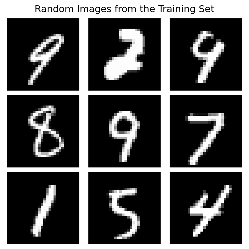
The images are of handwritten digits that look like this:
import matplotlib.pyplot as plt

N_ROWS = N_COLS = 3
out_path = './mnist_random_image_grid.png'

plt.ioff()
fig,ax = plt.subplots(N_ROWS, N_COLS, figsize=(8,8))
for i in range(N_ROWS):
    for j in range(N_COLS):
        idx = np.random.randint(low=0, high=x_train.shape[0])
        ax[i,j].imshow(x_train[idx], cmap='gray')
        ax[i,j].axis('off')
fig.suptitle("Random Images from the Training Set", fontsize=22, y=.98)
fig.tight_layout()
fig.savefig(out_path);
Since this is a supervised learning task, the data instances are labeled. The learning task is to predict the correct label out of the 10 possibilities.
In the y_train and y_test objects, you will see 10 dimensions for each data instance.
For each of these records, one of the ten dimensions will be a 1 and all others will be a 0.
You can verify this with the following assertion:
assert np.all(y_test.sum(axis=1) == 1)
Finally, you can view the distribution over true class labels to see that this dataset is relatively balanced.
import altair as alt
import pandas as pd

df = pd.DataFrame(y_test.sum(axis=0), columns=['Count'])
df.index.name = 'Class'
df.reset_index(inplace=True)

alt.Chart(df).mark_bar().encode(
    x='Count:Q',
    y="Class:O",
    tooltip=['Class', 'Count']
).properties(height=300, width=500)
2Fit a Baseline
Before training a model, it is useful to set a baseline. A common baseline for classification tasks is the majority-class classifier, which measures what happens when all of the data instances are predicted to be from the majority class. This pattern is demonstrated in our NLP tutorial. However, for the MNIST dataset and the corresponding image classification task described above, the majority class-classifier will lead to a baseline model that predicts correctly just over 10% of the time. This is not a very useful baseline. Instead, let's build a feedforward neural network to compare to a more advanced convolutional neural network you will build later.
3Configure Hyperparameters
These variables represent some training settings and the model's hyperparameters. Don't worry if you are unfamiliar with neural networks or what these words mean. If you do know what they are, feel free to experiment!
from tensorflow.keras import layers, Sequential, Input

num_pixels = 28 * 28
num_classes = y_test.shape[1]

kernel_initializer = 'normal'
optimizer = 'adam'
loss = 'categorical_crossentropy'
metrics = ['accuracy']

epochs = 3
batch_size = 32
verbose = 2
4Build a Baseline Model
Next, let's construct a Keras model adding layers.
The Keras layers apply matrix operations to data as it moves toward the output layer of the neural network.
In this case, we use two Dense layers. Dense means they are feed-forward, fully-connected layers.
model = Sequential()
model.add(layers.Dense(
    num_pixels, input_dim=num_pixels,
    kernel_initializer=kernel_initializer,
    activation='relu'
))
model.add(layers.Dense(
    num_classes,
    kernel_initializer=kernel_initializer,
    activation='softmax'
))
model.compile(loss=loss, optimizer=optimizer, metrics=metrics)
5Train Your Model
To work with the feed-forward network you need to reshape the images.
This is done by flattening the matrix representing the images into a one-dimensional vector with length num_pixels.
Notice that this is the same value as the input_dim of the first layer in the neural network you defined in the last step.
Once the data is ready, we can pass it to the model.fit function and train a neural network.
_x_train = x_train.reshape(x_train.shape[0], num_pixels).astype('float32')
_x_test = x_test.reshape(x_test.shape[0], num_pixels).astype('float32')
history = model.fit(
    _x_train, y_train,
    validation_data = (_x_test, y_test),
    epochs = epochs,
    batch_size = batch_size,
    verbose = verbose
)
6Evaluate the Baseline
After training the model you will want to evaluate its performance to see if it's ability to generalize is improving:
scores = model.evaluate(
    x_test.reshape(x_test.shape[0], x_test.shape[1] * x_test.shape[2]).astype('float32'),
    y_test,
    verbose=0
)
categorical_cross_entropy = scores[0]
accuracy = scores[1]
msg = "The model predicted correctly {}% of the time on the test set."
print(msg.format(round(100*accuracy, 3)))
7Save and Load Keras Models
Like all software development, it is important to create robust processes for checkpointing, saving, and loading.
This is even more important in computer vision, as model training can be expensive.
Luckily, Keras provides utilities for saving and loading models.
For example, you can save the model architecture, model weights, and the traced TensorFlow subgraphs of call functions with a simple model.save API.
Later you will see how to incorporate this into your flows which will help you train and make predictions with models in any environment you need to.
location = 'test_model'
model.save(location)
Using model.load with the same location will then reload the same model object state:
new_model = keras.models.load_model(location)
scores = model.evaluate(
    x_test.reshape(x_test.shape[0], x_test.shape[1] * x_test.shape[2]).astype('float32'),
    y_test,
    verbose=0
)
assert scores[1] > .96, "Model should be doing better after two epochs."
To learn more about your options for saving and loading Keras models please see this guide. It describes cases like how to save to the Keras H5 format instead of the newer SavedModel format and how to save and load only model weights.
In this lesson, you explored the MNIST dataset and built a high-accuracy baseline model. In the next lesson, you will build a convolutional neural network model to see how its performance compares to the baseline. See you there!